How We Made Multilingual Embeddings Work at 60,000 Queries a Second

At our scale, an embedding model has to be nearly free to run and still smart enough to be worth running. Here's how we got both.

Multilingual embeddings at 60,000 queries a second — recovering most of the quality distillation usually throws away, running at machine speed at a fraction of the cost

Abnormal is in the business of stopping cybercrime—an industry where detection speed and coverage are the difference between stopping an attack and explaining one after the fact. Email attacks don’t wait, and each one is a race.

A single missed business email compromise can mean a finance team wiring seven figures to an attacker impersonating their CEO, or an employee handing over credentials to a vendor that doesn’t exist. At Abnormal, our job is to understand what a message is actually trying to do—and act on it—before anyone can click a link or reply to a fraudulent request.

Natural Language Processing (NLP) is how we reason about that intent. But the best embedding models¹ force a brutal tradeoff: exceptional semantic understanding versus speed and scale.

This post covers how we eliminated that tradeoff in early 2025. We now run deep-quality text understanding across every message we see, at a scale most NLP systems aren’t built to operate in.

The Constraint

At peak, Abnormal processes over 60,000 messages per second²—all part of the billions of emails we handle daily. Our goal was to embed all of it and hand our models a dense signal on every message. However, that’s more than any detection engine can realistically afford at this volume.

This presents a classic detection tradeoff between cost and coverage: the signals worth the most tend to cost the most to produce. Running heavyweight transformer encoders against full traffic that early in the pipeline was computationally out of the question. So the usual compromise is to run NLP late and reserve embeddings for the traffic most likely to carry an attack, accepting that some signal is left on the table everywhere else.

That compromise has a downside. The most damaging attacks we see—CEO impersonation, vendor fraud, business email compromise—often carry no malicious link, no attachment, and no known-bad sender. Nothing for a payload-based filter to catch. The only thing that gives them away is intent, and reading intent takes real NLP—exactly what we couldn’t afford to run on every message.

If we could move real text understanding to the front of the pipeline, at full traffic and inside a real-time latency budget, we could act on semantic risk early instead of late. To get there, we needed one thing: an embedding model fast enough to be effectively free at 60,000 queries per second, yet smart enough to be worth running.

The Seed: A Static Embedding Model

We started by distilling³ a tuned multilingual encoder using model2vec. model2vec collapses a full transformer encoder into a set of static token embeddings: instead of a forward pass through stacked attention layers at inference time, embedding a piece of text becomes a lookup-and-pool operation over precomputed token vectors. The result is a ~128MB static embedding - far smaller than a typical open-source encoder.

Paired with a bespoke scoring implementation for this pooling model, we achieved embedding inference in microseconds. This makes embedding a 60,000 queries per second stream feasible.

However, a static, bag-of-tokens representation⁴ gives up the contextual and multilingual nuance a full transformer captures. Our evals confirmed this: the base static model trailed its heavier counterparts on semantic quality. Our question became: how could we recover that quality without giving up the speed?

The Idea: Distill Judgments, Not Weights

Instead of replacing the fast model, we taught it to behave like a bigger one. We built a pipeline that transfers knowledge from two teachers—a state-of-the-art (SoTA) multilingual embedding model and an LLM used for text normalization—into our student, the lightweight static embeddings model.

1. Adversarial text normalization with an LLM. Attackers deliberately obfuscate text to evade NLP (think Unicode look-alikes, injected whitespace, homoglyphs, broken word boundaries, etc.), and emails are often padded with prepended/appended cruft that has nothing to do with intent. We used an LLM to normalize a multilingual corpus of known-malicious emails drawn from our proprietary threat intelligence, de-identified across customers, back into clean canonical text, leveraging the LLM’s encyclopedic knowledge to undo obfuscation before anything downstream sees it.

2. Teacher similarities from a SoTA embedding model. We embedded the cleaned corpus with a strong multilingual embedding model (much larger than our tuned encoder used for model2vec distillation), then sampled pairs of texts and recorded the cosine similarity⁵ each pair received under the teacher.

The student and teacher live in different embedding spaces with different dimensionalities, so we couldn’t just regress one embedding onto the other. To get around this, we don’t distill the vectors; we distill the relationships. We train the student so that the scaled cosine similarity it assigns to a pair matches what the teacher assigned to that same pair.

Architecturally (see Figure 1), the model2vec table is a frozen vocab_size × N matrix of static token embeddings. We learn a single shared-weight (siamese) N × N transformation over those embeddings, compute cosine similarity on the transformed student vectors, and minimize the gap to the teacher’s similarity. Only the N × N matrix is trained; the base table stays frozen during optimization.

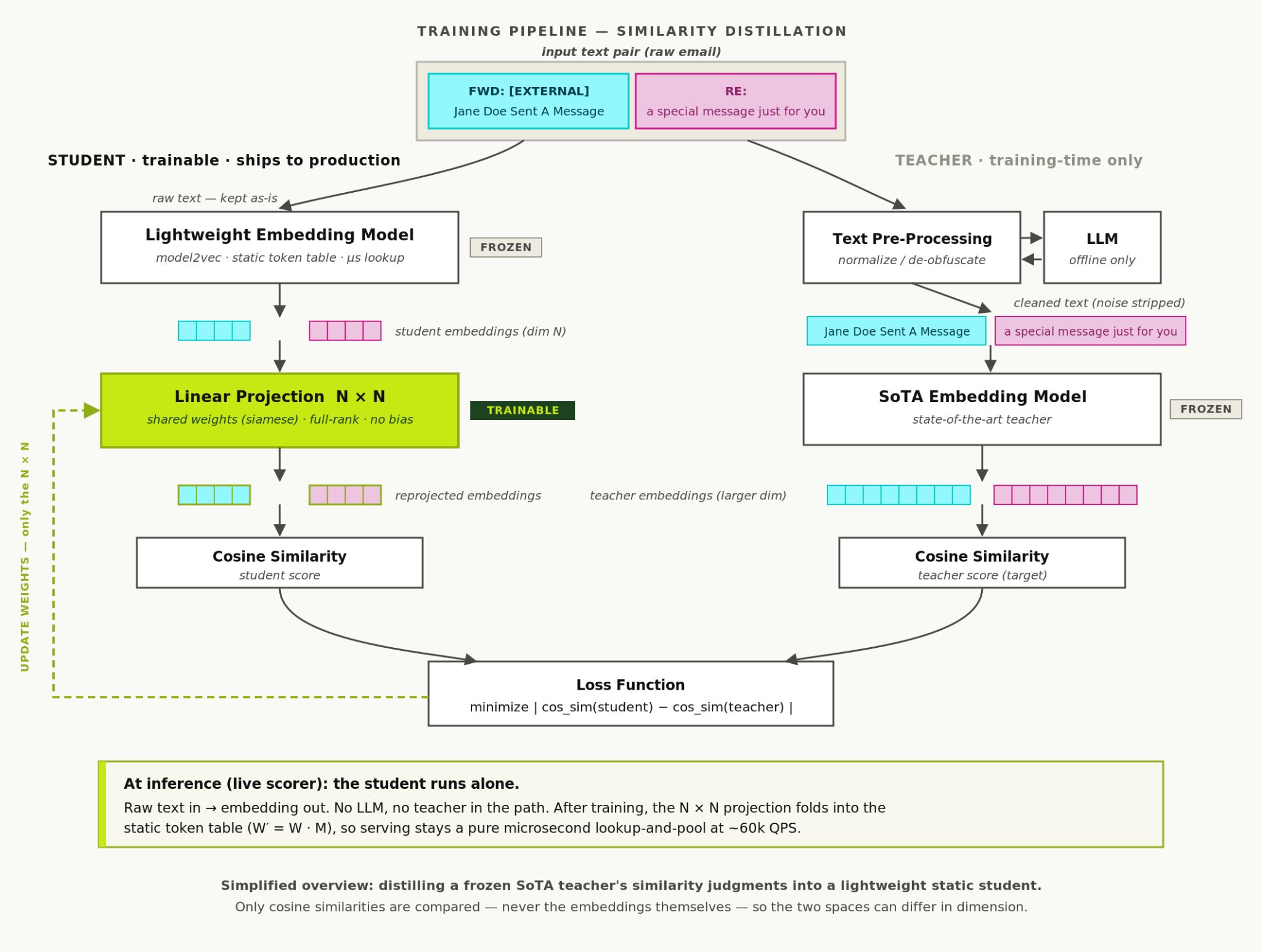
Figure 1: Training Pipeline for Similarity Distillation

We can elegantly combine the trained weights back into the original model, without an increase in model size!

Because embedding is a linear, bag-of-tokens operation, transforming each token vector then pooling is identical to pooling then transforming. So, once training converges, we multiply the learned N × N matrix back into the frozen table and get a new vocab_size × N static table. The transformation collapses into the weights—inference stays a pure lookup-and-pool at microsecond cost, with zero added parameters at serving time⁶.

As a result, the lightweight model inherits the teacher’s judgment of which texts are semantically close and which aren’t, including cross-lingual structure it never learned on its own, all while keeping microsecond inference⁷.

The Results

We evaluated on a labeled in-house multilingual retrieval dataset, comparing three models:

• Baseline – our static model prior to similarity distillation.

• Tuned – the same model after being taught via similarity distillation.

• Benchmark – a ~600M parameter open-source model (~19× larger), used as the quality benchmark.

We measured quality with two standard retrieval metrics:

• NDCG@10 (Normalized Discounted Cumulative Gain at cutoff 10) – rewards putting the most relevant results at the top of the first 10.

• MAP@10 (Mean Average Precision at cutoff 10) – rewards retrieving relevant results across the first 10, weighted toward earlier hits.

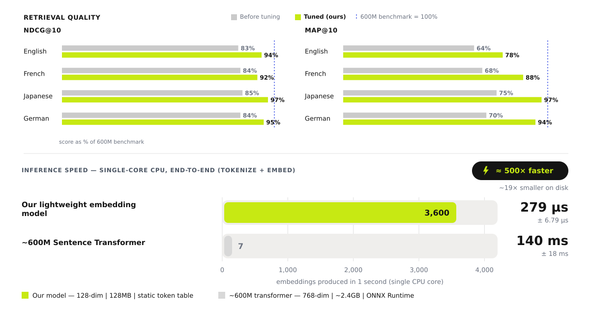
Figure 2: Model Performance Gains Post Distillation

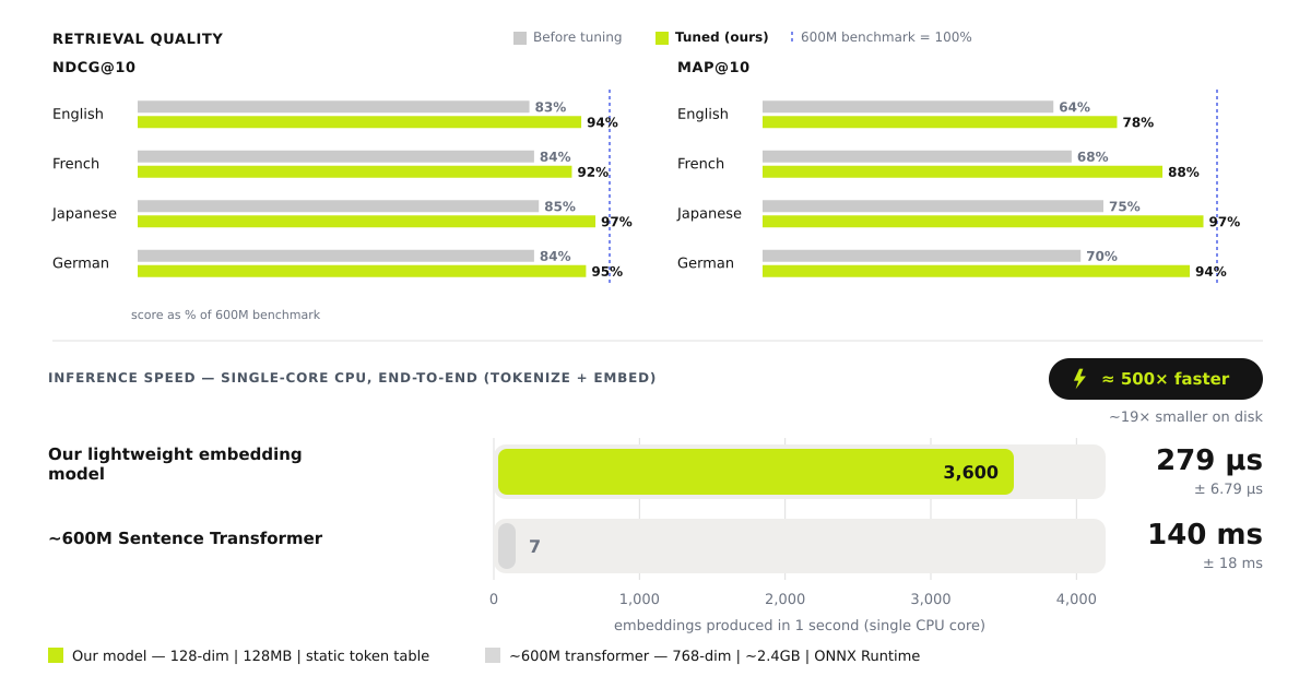
We found that the tuned model closed most of the gap. From the same 128MB base, similarity distillation recovered 92–97% of the benchmark on NDCG@10 and 78–97% on MAP@10⁸, all while running in microseconds.

Why This Matters

With this distillation technique, we can now run deep text understanding on every message, changing where detection can actually happen. Inbound messages now carry a semantic signal computed at the front of the pipeline, so our downstream detectors reason about what an email is trying to do from the very first pass, instead of waiting for a heavyweight model to weigh in on a sampled subset near the end.

That compounds in a few ways:

• Scalable protection - Microsecond inference lets us embed the full ~60k-QPS inbound stream instead of rationing text understanding to a fraction of traffic.

• Faster detection - Generating semantic embeddings at the front of the pipeline lets us surface risk before a user can even engage with a malicious message.

• Multilingual coverage - Because both teacher models were cross-lingual, that structure transfers into the static model—critical for our many customers who run operations across different languages.

• Resource efficiency - We removed compute cost as the blocker for NLP inference, making advanced text analysis practical at production scale.

Final thoughts

Bigger isn’t always better. With the right distillation strategy, a small model can carry the judgment of a much larger one, sparing us the classic tradeoff between the quality of a big model and the coverage of a cheap one. That’s the difference between stopping an attack and explaining one—at 60,000 messages a second.

1. An embedding turns a piece of text into a vector of numbers, so that texts with similar meaning land near each other.

2. Metric measured by our internal dashboards that measures queries per second our message scoring service receives

3. Distillation is the practice of transferring what a large model knows into a smaller, cheaper one.

4. Treating text as an unordered set of tokens, ignoring word order.

5. How aligned two vectors are.

6. A note on what this is (and isn’t): this is a full-rank linear reprojection of the embedding space, folded back into the static table – not LoRA. LoRA applies a low-rank update (ΔW = B·A, with a chosen bottleneck rank r ≪ N) that persists as an additive adapter. Our transform has no rank bottleneck (the N × N matrix is full-rank) and isn’t additive. We merge it directly into the frozen weights, which is closer to weight reparameterization than to adapter-based fine-tuning.

7. Why a global reprojection instead of tuning the table directly? We could have made every entry of the vocab_size × N table trainable—that's strictly more expressive. But, the distillation signal (pairwise similarities on sampled pairs) is weak and only touches tokens that appear in the corpus, so direct tuning would overfit those tokens while leaving the long tail stranded in the original space. A single shared N × N map recalibrates every token coherently, including ones never seen in training, with a tiny, stable set of parameters. It's the same principle behind linear cross-lingual embedding alignment; for reshaping one space's similarity structure toward another's. Additionally, our testing indicated that a global linear transform is both sufficient and far simpler than moving thousands of embeddings independently.

8. Retrieval quality was measured on a held-out, labeled multilingual dataset (English plus French, Japanese, and German). We treat the ~600M benchmark model’s nearest-neighbor rankings as ground truth: for each message, its top-100 neighbors under the benchmark define relevance. We then retrieve each candidate model’s top-10 neighbors and score them against that reference — MAP@10 for how relevant the retrieved neighbors are, NDCG@10 for how well their ordering matches the benchmark’s. Scores are reported per language as a percentage of the benchmark’s, so “recovered 92–97%” means the tuned model reproduced that fraction of the benchmark’s retrieval quality.

Why is English’s lift smaller? Most of our data is in English, so the benchmark’s English set is larger and more diverse, more candidates means harder retrieval and lower scores. The smaller non-English sets have fewer distractors, which flatters their numbers. We treat the English figures as conservative, real-world estimates.